Forced Response Surface

Consider a mechanical system of the type

$\mathbf{M} \mathbf{\ddot{y}} + \mathbf{C} \mathbf{\dot{y}} +\mathbf{K}\mathbf{y} +\mathbf{f}(\mathbf{y}, \dot{\mathbf{y}}) =\epsilon \mathbf{f}^{ext} \cos(\Omega t)$

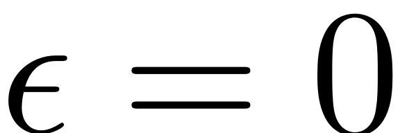
Here, $\mathbf{f}$ is a nonlinear function. We assume that the autonomous system ( $\epsilon=0$ ) admits a hyperbolic fixed point $(\mathbf{y},\dot{\mathbf{y}})=\mathbf{0}$ . The under the addition of the harmonic excitation, the fixed point is perturbed as a periodic orbit of the same stability type. When $\epsilon$ is increased, bifurcations of periodic orbits can be observed. We have forced response surface (FRS) of periodic orbits under the variations in forcing frequency $\Omega$ and forcing amplitude $\epsilon$ . The FRS is a two-dimensional manifold of periodic orbits. Along the surface, its ridge is a curve of local maximum under varying $\Omega$ but fixed $\epsilon$ . In other words, a ridge is defined as a family of maximum of FRCs. Likewise, a trench is defined as a family of minimum of FRCs.

To effeciently extract the FRS, we perform model reduction via spectral submanifolds (SSMs). In particular, a periodic orbit of the original high-dimensinal system is simplified as a fixed point of the SSM-based reduced-order model (ROM). For systems without internal resonances, we can extract the FRS analytically. For systems with internal resonances, one can use two-dimensional parameter continuation of fixed points of the SSM-based ROM to extract the FRS of periodic orbits.

Ridges and trenches characterize the main features of the FRS. Thus, it is instructive to extract the ridges and trenches without computing the surface. This gives a more efficient charaterization of the FRS. We note that ridges and trenches are stationary periodic orbits along forced response curves with fixed forcing amplitudes. This suggests that one can define proper optimization problem to extract the ridges and trenches. Indeed, one can use successive continuation of first-order necessary conditions to extract ridges and trenches.

Detailed treatment of the theory and algorithm extracting FRS and ridges and trenches can also be accessed in the related publication (Li, Jain & Haller, 2024).

Contents

Computation of FRS

After setting up the dynamical system, and the SSM object S, the FRS can be extracted by using the following built-in method:

S.extract_FRS(oid,modes,order,mFreqs,parRange,outdof,optdof,scale_state,scale_obs,varargin)

The input arguments are as follows

We note that we can set the method in FRSOptions to be 'level set' or 'continuation'. With 'level set', we extract the FRS analytically. With 'continuation', a two-dimensional continuation algorithm is used to extract the FRS.

Computation of ridges and trenches

After setting up the dynamical system, and the SSM object S, the FRS can be extracted by using the following built-in method:

S.extract_ridges_trenches(oid,resonant_modes,order,mFreqs,parRange,outdof,optdof,varargin)

This function extract the damped backbone curve (defined as amplitude resonance) of reduced-order model (in slow phase) as optimization problem of fixed points. Note that this backbone curve will be slightly deviated from the one for a given physical coordinate because the contribution of non-autnomous SSM to the response in physical coordinates. Each equilibirum point corresponds to a periodic orbit in full system. The continuation here starts from the guess of initial solution (for fixed point, adjoints are initialization-free).

The input arguments are as follows

Examples

Published with MATLAB® R2023a